 GambleLore
Understanding Variance in Sports Betting for 2026
Variance in sports betting describes the short-term fluctuations between expected outcomes and actual results, even when a bettor consistently identifies positive expected value opportunities. In 2026 these swings remain a core challenge for anyone wagering on football, the NBA, or tennis. Bettors who focus solely on long-term edges without accounting for variance often misinterpret normal downswings as strategy failures and make costly adjustments. This article explores variance in depth, provides concrete measurement techniques, and delivers actionable bankroll rules tailored to the 2026 calendars of the three most variance-prone sports. Understanding variance begins with recognizing that it is a statistical property separate from your betting edge; a positive edge guarantees profit only over large samples, while variance dictates how much your bankroll will oscillate along the way.
Why Variance Hits Football, NBA, and Tennis Bettors Hardest
Football produces low-scoring matches where a single defensive error or referee decision can swing the result by multiple goals. The 2026 season includes an expanded international schedule that increases fixture congestion and player fatigue, amplifying outcome randomness. The NBA features high possession counts and three-point variance, meaning even strong player-prop models experience nightly swings of 15 or more points. Expanded play-in tournaments and load-management strategies in 2026 add further unpredictability. Tennis matches consist of independent points and sets that create binary outcomes; a single tiebreak or service break can erase hours of statistical dominance. Grass, clay, and hard-court transitions during the 2026 Grand Slam and Masters 1000 circuit further heighten surface-specific variance. These structural characteristics make variance more pronounced than in higher-scoring or more predictable sports such as baseball or hockey.
Real-World Examples of Variance Swings Across Sports
In football, a bettor backing under 2.5 goals at even money may see the match finish 0-0 for 90 minutes only for two late goals to push the total to 3. Historical data from the Premier League shows that roughly 28 percent of matches decided by one goal flip the under/over result in the final 10 minutes. In the NBA, a sharp bettor targeting a star’s points prop at 28.5 may watch that player finish with 22 points after an unusually cold shooting night despite 18 field-goal attempts. Across a 10-game sample, such variance can produce five losses even when the underlying projection remains accurate. Tennis provides the clearest illustration: a top-10 player favored at -180 may lose a deciding-set tiebreak 7-6 after winning 62 percent of service points, turning a high-probability bet into a loss. Another example involves an NBA moneyline bet on a favorite at -150; even with a 60 percent true win probability, a three-game losing streak occurs roughly once every eight series due to random variance alone. In tennis, a bet on a player to win in straight sets can lose despite dominating possession of points if the opponent capitalizes on two break opportunities in tiebreaks. These examples demonstrate that variance operates independently of edge and must be measured separately.
Step-by-Step Methods to Measure and Track Variance
Begin by exporting at least 300 historical bets from your chosen leagues, recording stake, odds, closing line, and actual profit or loss. Calculate the standard deviation of returns using a spreadsheet formula: subtract the mean return from each individual return, square the result, average the squares, and take the square root. Compare this figure to your expected value per bet. Next, import current 2026 odds daily and calculate implied probabilities, then subtract your model’s estimated true probability to quantify closing-line value. Maintain a rolling 50-bet window to monitor when realized variance exceeds two standard deviations from your long-term average. Tools such as Google Sheets or dedicated tracking software allow automatic alerts when variance metrics breach thresholds. Finally, segment results by sport and bet type to identify which markets exhibit the highest volatility during the current season. Advanced users can apply the Sharpe ratio adapted for betting by dividing average profit per bet by the standard deviation, providing a risk-adjusted performance metric that highlights when variance is eroding returns more than expected.
Practical Bankroll Adjustments and Session Rules
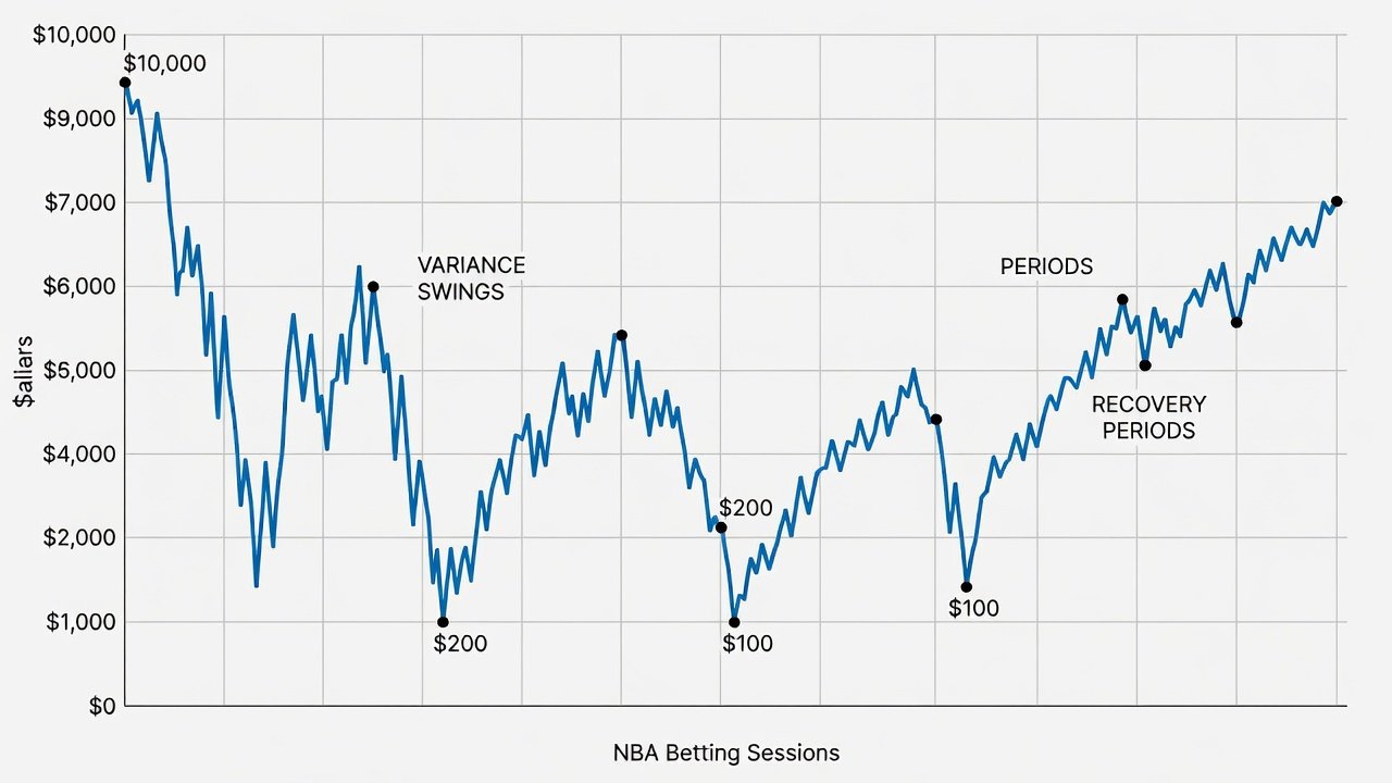
Reduce unit size to 1 percent of total bankroll during periods of elevated fixture density, such as the NBA’s February trade deadline or tennis’s clay-court swing. Increase back to 2 percent only after variance metrics return inside one standard deviation for 30 consecutive bets. Establish hard session rules: end betting after three consecutive losses or when daily exposure reaches 5 percent of bankroll. These limits prevent emotional escalation and protect capital for higher-edge opportunities later in the 2026 season. Review weekly variance reports and adjust stake sizes downward if the current standard deviation is more than 30 percent above your historical baseline. For instance, if your bankroll sits at $10,000 and standard deviation spikes, drop stakes from $200 to $100 per bet until stability returns. Document every adjustment in your tracking log so you can analyze whether the changes improved long-term profitability.
Comparing Variance Across the Three Sports
Football variance tends to cluster around match totals and Asian handicaps because of low event frequency. NBA variance is highest in player props and quarter betting due to small sample sizes within games. Tennis variance peaks in set and game betting where individual points carry outsized influence. Bettors who spread action across all three sports should calculate separate standard deviations for each rather than using a blended figure, as the risk profiles differ substantially.
Common Mistakes to Avoid
- Chasing losses by doubling stakes after downswings without recalculating variance
- Declaring a model broken after only 50 to 80 bets when sample size remains too small
- Switching between football, NBA, and tennis without recalculating sport-specific standard deviations
- Ignoring external factors such as schedule congestion or surface changes that legitimately increase variance
- Overlooking the impact of line movement on true variance calculations
Short FAQ on Variance Misconceptions
When should I stay the course versus adjusting strategy?
Stay the course if your edge and closing-line value remain positive after at least 200 tracked bets. Adjust only when league rules, player availability patterns, or market efficiency change materially during the 2026 season.
Does variance ever disappear for professional bettors?
No. Even the most successful bettors experience variance; professional management focuses on surviving swings rather than eliminating them.
Can I reduce variance by betting only overs or only unders?
Market selection may slightly alter variance magnitude but cannot remove it. Diversifying across uncorrelated markets within the same sport offers modest reduction.
How many bets are needed before variance becomes manageable?
Most statisticians recommend a minimum of 300 to 500 bets per sport before drawing firm conclusions about edge versus variance.
Additional authoritative data sources include the Premier League official site, NBA.com, and ATP Tour for historical results and schedule information. Consistent tracking combined with disciplined bankroll rules allows bettors to navigate 2026 variance without abandoning sound strategies.

No comments yet. Be the first!